Text in English below.

Etant donné que je suis actif sur 144 MHz en EME (terre-lune-terre), j’ai besoin de puissance RF. Après une version 300W, puis 600W, j’ai construit un SSPA (Solid State PA) de 1 kW+ en 2017 (une vidéo relative à cet ampli est disponible ici). Il est basé sur un kit de Jim, W6PQL (matériel très fiable). Le transistor utilisé est un BLF188XR. Cet ampli a parfaitement fonctionné jusque mi juin 2023. Durant une émission en mode numérique et par journée chaude (31°C), il a cessé de fonctionner ! Pour limiter les pertes, le transverter 28 <> 144 MHz et l’ampli sont disposés dans un abri au pied de mon pylône, dans le jardin. L’abri n’est pas climatisé, si bien que par les journées chaudes, le refroidisseur est déjà à 30°C+ sans avoir même émis un watt RF…

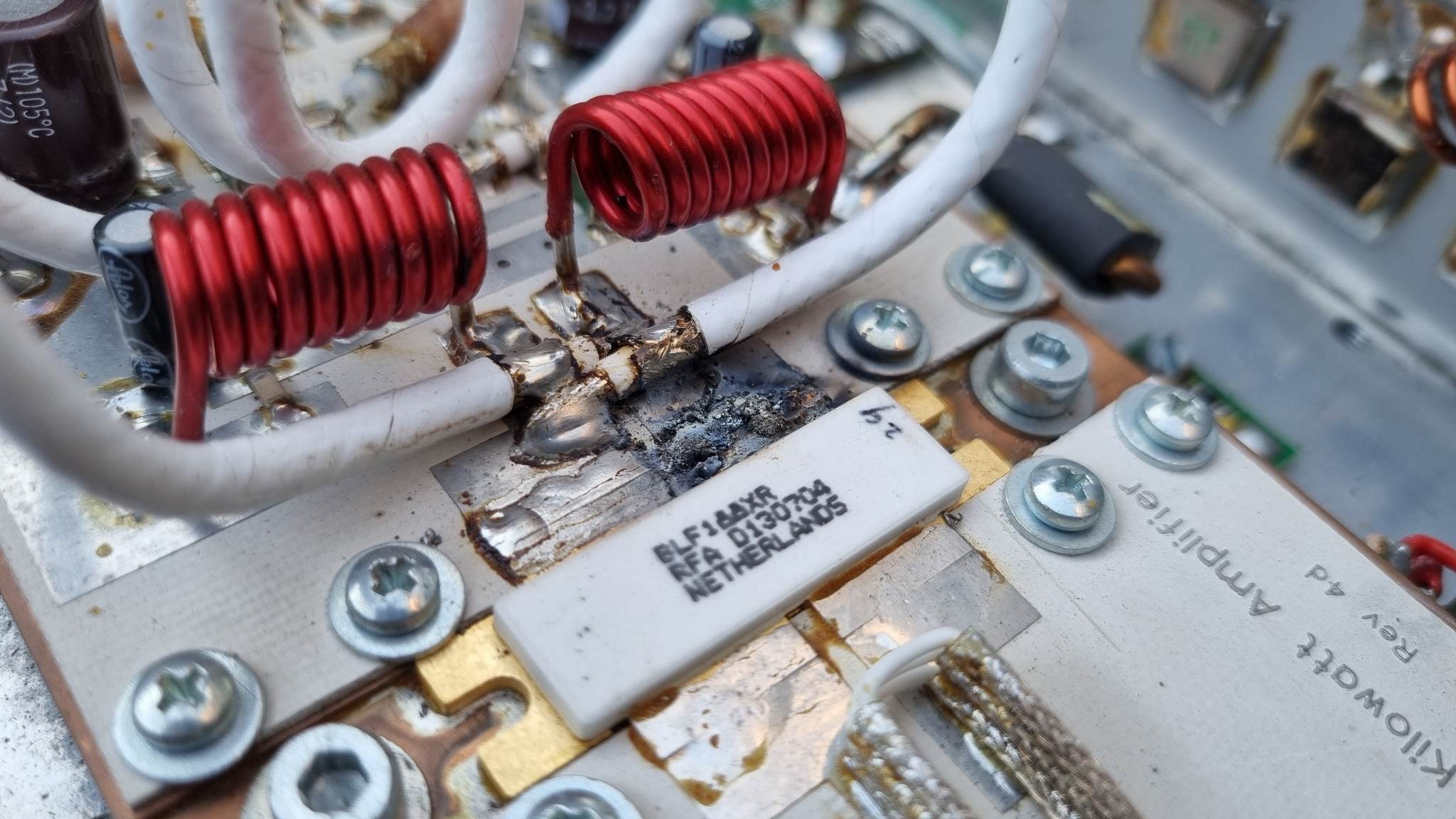
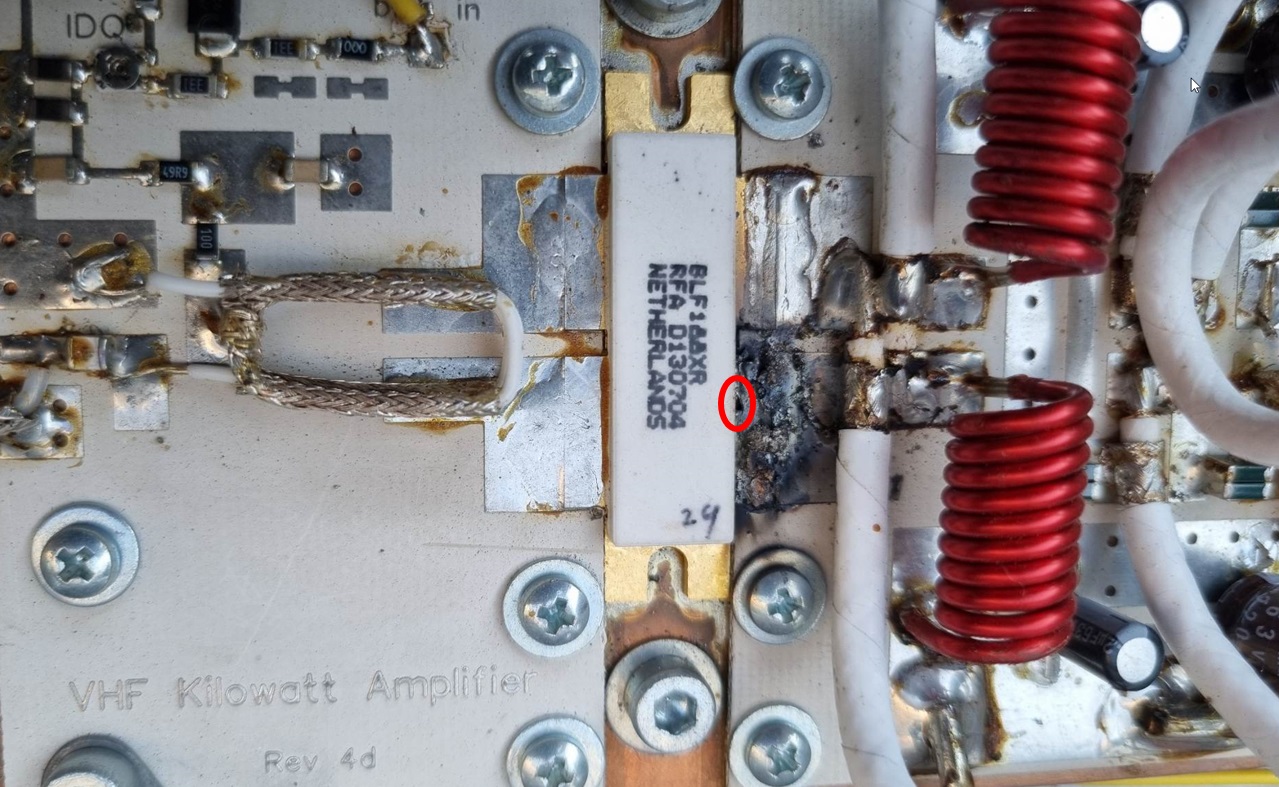
L’examen de l’ampli après sa défaillance montre une fonte partielle du drain droit et il y a un petit trou dans le drain, juste à la base du boîtier du transistor (voir photo). La vérification à l’ohm-mètre indique que le drain droit n’est plus en contact avec le PCB. A ce moment-là, je me dis qu’il faudra remplacer le transistor, ce qui ne me ravit pas. Un transistor neuf coûte 250€ et l’opération de dessoudage et ressoudage du transistor sur la semelle en cuivre n’est pas une opération aisée !

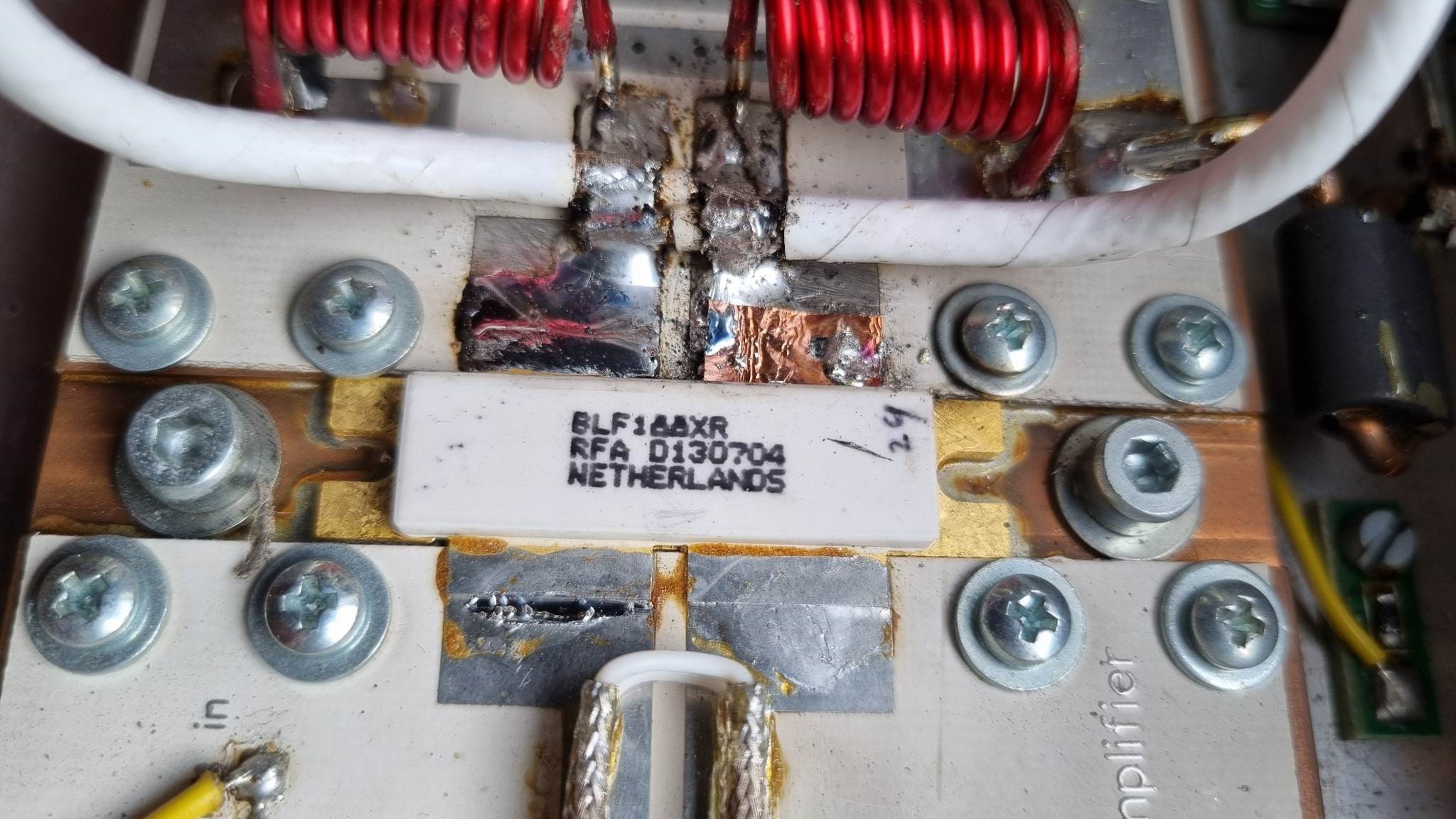
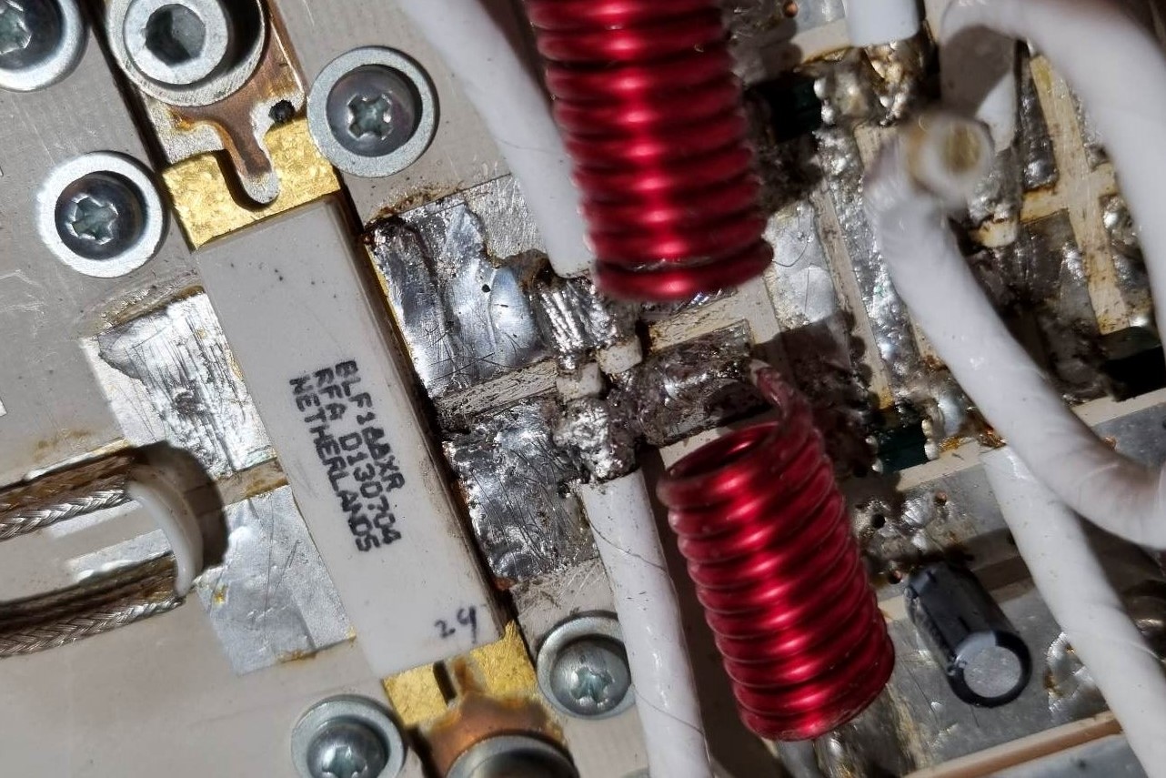
Sans trop y croire donc, j’ai essayé de récupérer autant que possible le drain fondu. Cette opération de “récupération” passait par le retrait (même partiel) de la forte oxydation du drain liée à la fonte. J’ai ensuite refait une soudure sommaire, juste pour rétablir le contact entre le drain défaillant et le PCB. Ensuite, j’ai mesuré à l’ohm-mètre la résistance entre les gates du transistor (l’ohm-mètre ne doit pas envoyer plus de 3-4 V) et la source du transistor qui se trouve à la masse (soudée sur le refroidisseur). Ce, en ayant pris soin de dessouder les composants périphériques qui mettent en contact direct (DC) les gates à la masse. La mesure indique une résistance infinie. C’est bon signe, les gates ne sont pas en court-circuit. Idem pour les drains (mesure de la résistance drains – masse) et la résitance est de l’ordre du mégohm (de mémoire), ce qui est également bon signe. Le transistor ne serait-il pas claqué ? Manipulation suivante (après ressoudage des composants périphériques) : mise des drains sous tension nominale (52V) et application de la tension de polarisation sur les gates (environ 2V). Le courant (de repos) dans les drains indique 3A, ce qui est également bon signe. J’ai donc fait une soudure plus sérieuse du drain droit (avec application d’un feuillard en cuivre, voir photo) et renforcé quelques autres soudures. A l’application d’une puissance RF en entrée, et après avoir réaligné le courant de repos à 2A, l’ampli sort à nouveau près de 1,2 kW. Contre toute attente, le transistor n’était donc pas claqué !

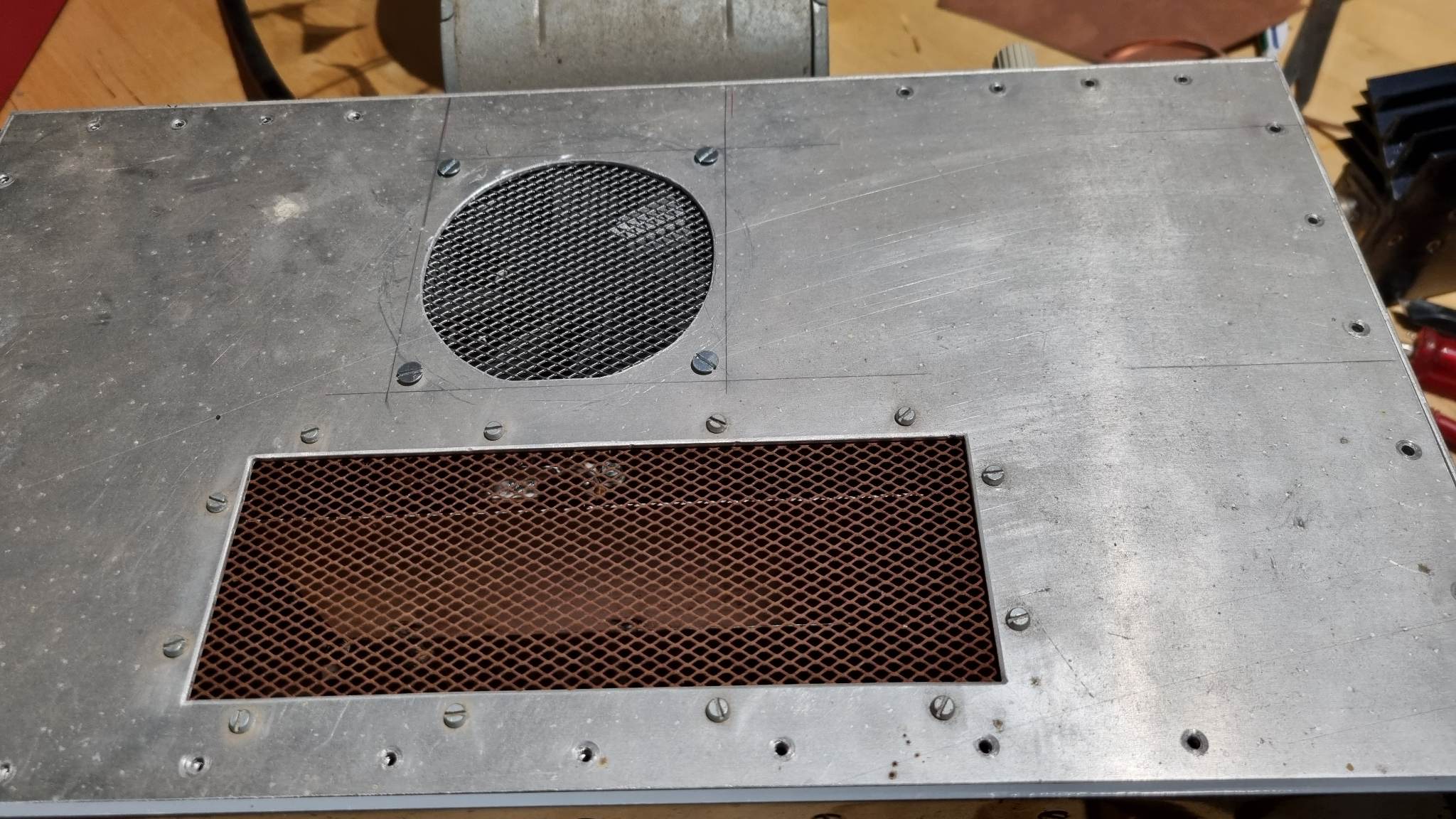
J’attribue la défaillance, soit à une dégradation graduelle de la soudure des drains en raison de la température (dissipation thermique), jusqu’à rupture et arc électrique, ou à la présence d’un insecte dans l’ampli (pour rappel, il est dans le jardin) qui aurait amorcé un arc électrique. Pour rendre durable la réparation, j’ai revu un peu la gestion du refroidissement. En plus de la ventilation forcée déjà en place sur le refroidisseur, j’ai mis un ventilateur au-dessus de PCB, pour le refroidir et dissuader la présence d’un insecte. Sur la carte de contrôle de W6PQL (V6), j’ai appliqué 3,2V (au lieu de 2,8V) sur le “test point 1”, afin de diminuer le seuil d’enclenchement/maintien de la ventilation forcée (ventilateurs).

Since I’m active on 144 MHz in EME (earth-moon-earth), I need RF power. After a 300W, then a 600W version, I built a 1kW+ SSPA (Solid State PA) in 2017 (a video relating to this amp is available here). It’s based on a kit from Jim, W6PQL (very reliable equipment). The transistor used is a BLF188XR. This amp worked perfectly until mid-June 2023. During a digital transmission on a hot day (31°C), it stopped working! To limit losses, the 28 <> 144 MHz transverter and the amplifier are placed in a shelter at the foot of my tower, in the garden. The shelter is not air-conditioned, so on hot days the heatsink is already at 30°C+ without having emitted even one RF watt…

Examination of the amp after its failure shows partial melting of the right drain and there’s a small hole in the drain, just at the base of the transistor case (see photo). A check with the ohm-meter shows that the right drain is no longer in contact with the PCB. At this point, I say to myself that I’m going to have to replace the transistor, which I’m not happy about. A new transistor costs 250€ and unsoldering and re-soldering the transistor to the copper plate is not an easy operation!

Without really believing in it, I tried to recover as much of the melted drain as possible. This “recovery” operation involved removing (even partially) the heavy oxidation from the drain due to melting. I then did some rough soldering, just to re-establish contact between the faulty drain and the PCB. Then I used an ohm-meter to measure the resistance between the gates of the transistor (the ohm-meter shouldn’t send more than 3-4 V) and the source of the transistor, which is at earth (soldered onto the heatsink). I took care to desolder the peripheral components that put the gates in direct contact (DC) with earth. The measurement indicates infinite resistance. This is a good sign that the gates are not short-circuited. The same goes for the drains (measurement of the resistance drains – earth) and the resistance is of the order of one megohm (from memory), which is also a good sign. Could the transistor still be working? Next step (after re-soldering the peripheral components): apply nominal voltage (52V) to the drains and apply the bias voltage to the gates (about 2V). The (quiescent) current in the drains indicates 3A, which is also a good sign. So I did a more serious soldering of the right drain (with application of a copper strip, see photo) and reinforced a few other solder joints. When RF power was applied to the input, and after realigning the quiescent current to 2A, the amp once again produced almost 1.2 kW. So, against all expectations, the transistor wasn’t blown!

I attribute the failure either to a gradual degradation of the soldering of the drains due to the temperature (heat dissipation), until it broke and arced, or to the presence of an insect in the amp (as a reminder, it’s in the garden) which initiated an electric arc. To make the repair sustainable, I’ve reviewed the cooling management a little. In addition to the forced ventilation already in place on the heatsink, I put a fan on top of the PCB, to cool it and dissuade the presence of an insect. On the W6PQL control board (V6), I applied 3.2V (instead of 2.8V) to “test point 1”, in order to lower the threshold for switching on/holding the forced ventilation (fans).

SPACE

For the digital modes traffic, I run WSJT-X on a Raspberry Pi (4B). So, no need to devote a “big” computer for that purpose, the Raspberry does the job perfectly well, and for less power consumption and noise. For my 144 MHz moonbounce operations, I wanted a simple system to drive my existing ERC-3D rotator controller (by DF9GR). That model is now obsolete but works flawlessly and I wanted to keep it as-is, without changing anything. The ERC-3D is linked to azimuth (Yaesu G650) and elevation (Kenpro KR500) antenna rotators.

The search for a ready made program I did on the Internet was not successful, since I wanted to keep as-is my exisiting system. Having in mind that WSJT-X provides an azel.dat file including the coordinates of the moon, I decided to write a program to extract these data and to use them to command my ERC-3D, in first place to track the moon.

To be able to do it, a prerequisite is to have Hamlib installed on the Raspberry. What is hamlib : “the Ham Radio Control Library –Hamlib, for short– is a project to provide programs with a consistent Application Programming Interface (API) for controlling the myriad of radios and rotators available to amateur radio and communications users”. To date the current hamlib version is 4.2. and can be downloaded here. How to install it on the Raspberry is out of the present scope, there a several tutorials on the Internet that clearly explain it (it is very easy).

Once Hamlib was installed, the program had to be written (it is available at the end of this post). It has been written in Python 3 and, since I’m not at all a programmer, it is my friend Didier (ON4KDV), who wrote the backbone of the program (many thanks to him !). I then customized it and added some features, a.o. the possibility to command the rotator controller not only to automatically track the moon but also to rotate/elevate the antennas wherever needed.

The program is named “Rotator Controller” and an icon placed on the desktop of the Raspberry allows to launch it easily. It opens in the command-line terminal.

Here is below how it works.

First you select the USB port to be used and then you have the choice :

• Manual rotation/elevation
• Automatic tracking of the moon, as from the azel.dat file out of WSJT-X
• Exit

We start first with the manual rotation/elevation. The possible options are self-explanatory. See also the code at the end, it provides many explanations (comments) too.

When the option “r” is selected, if it was elevated before, the antenna will come back to the horizon (0° elevation) and towards the wished azimuth. “s” will stop immediately any rotation/elevation.

On the example here, we set the azimuth to 113°. Then we ask for the position (“p”) and we see that the antenna is effectively well on Az. 113°.

Then we select “l” and we set Az. to 113° and El. to 10°. Requesting the position by typing “p”, we get well 113° Az. and 10° El.

To come back to the main menu, you have to exit (“e”) and restart the program. Before restarting the program, we must start first WSJT-X, so that the azel.dat file is available. We then restart the program and we select a USB port not already in use by WSJT-X (for the CAT for example).

We select “a” for the automatic moon tracking. We are prompted to set a “refresh duration”, it is the time interval (in minutes, but can be customized in seconds, see comments in the code) between two refreshes of the moon position (access to the azel.dat file in WSJT-X).

Every x (2 in the example) minutes, as per defined by the “refresh duration”, the moon position is derived from the azel.dat file, the antenna is rotated and elevated accoringly, and the actual antenna position (azimuth and elevation) is reported 5 seconds later.

If the moon is below the horizon, nothing happens and the program indicates “The moon is below horizon, antenna parked !”, and so on until the moon rises above the horizon. To  exit, press “CTRL” and “C”.

Here is the heavily commented python 3 program :

#!/usr/bin/python3
# coding: utf-8

# This script allows to rotate an antenna system either by manually typing in a heading (azimuth and/or elevation)
# you want the antenna to rotate to or by automatically tracking the moon azimuth and elevation.
# The Moon azimuth and elevation are extracted out of the file azel.dat provided by the WSJT-X suite.
# Beside WSJT-X, this script also makes use of the rotator controller daemon embedded in the Hamlib
# libraries. So, the prerequisites for this script to run are WSJT-X opened and running, and the
# Hamlib librairies installed on your Raspberry Pi.
# This script has been written in Python 3 by Didier, ON4KDV and Gaëtan, ON4KHG.
# My personnal system makes use of a Raspberry Pi 4B and an ERC-3D (DF9GR) antenna rotator controller.
# Both are linked with a USB (on the Raspberry Pi side) to RS232 serial (on the controller side) connection.
 
# First, import the time, system and subprocess functions needed in this script

import time
import os, sys
import subprocess

# Select the USB port of the Raspberry Pi onto which the rotator controller is connected.
# Normally, as WSJT-X is started beforehand, the USB0 port is already assigned for the CAT & PTT of WSJT-X.
# In my case, I usually select USB1, so, I type “1” below. 

usb_port=(input(“USB port to use (0-3) : “))
print()

if usb_port == “0”:

# The Rotctld(aemon) is opened with the command “rotctld -m 601 -r /dev/ttyUSB0 &”.
# -m 601 is related to the GS-232A rotator protocol.
# You could have to have to select another number according to the protocol and associated hardware in use on your side.
# The list of supported protocols can be obtained by typing “rotctld -l” in the terminal.
# ttyUSB0 is the serial port (USB0) of the Raspberry onto which the rotator controller is connected.

        subprocess.call(‘rotctld -m 601 -r /dev/ttyUSB0 &’, shell=True)

# And so on for the other USB ports.
         
elif usb_port == “1”:
         
        subprocess.call(‘rotctld -m 601 -r /dev/ttyUSB1 &’, shell=True)
         
elif usb_port == “2”:
         
        subprocess.call(‘rotctld -m 601 -r /dev/ttyUSB2 &’, shell=True)
         
elif usb_port == “3”:
         
        subprocess.call(‘rotctld -m 601 -r /dev/ttyUSB3 &’, shell=True)
         
# Select the working mode : manual, automatic (moon tracking) or exit.

Mode=(input(“MANUAL rotation/elevation, type m\nAUTOMATIC tracking, type a\nEXIT, type e\n\n”))

if Mode == “m”:

# If “m” is chosen, the manual rotation mode is selected.
   
    while (True):

# Then, select what you want to do : rotate/elevate the antenna, get its current position, stop the rotation in case
# of emergency or exit.
     
      Submode=(input(“\nROTATE antenna (azimuth only) and set elevation to 0°, type r\nROTATE and ELEVATE antenna (azimuth and elevation), type l\nGet current POSITION, type p\nSTOP, type s\nEXIT, type e\n\n”))
     
      if Submode == “r”:
         
# If “r” is selected, instruct towards which azimuth the antenna has to rotate. With this selection, if the antenna was previously elevated,
# it will be set back to 0° (no elevation) too.        
        
         az=(input(“\nRotate antenna to azimuth (°) : “))
         az=az.strip()
                 
# Build and execute the command “set_pos”. The default port used by the rotctld(aemon) is 4533.

         command_az=’echo “|\set_pos ‘ + az + ‘ 0” | nc -w 1 localhost 4533’
         os.system(command_az)

      elif Submode == “l”:

# If “l” is selected, you can set whatever azimuth and elevation angle.

         az=(input(“\nRotate antenna to azimuth (°) : “))
         az=az.strip()
         el=(input(“Elevate antenna to elevation (°) : “))
         el=el.strip()

         command_azel=’echo “|\set_pos ‘ + az + ‘ ‘ + el + ‘” | nc -w 1 localhost 4533’
         os.system(command_azel)
     
# If “p” to get the position of the antenne is selected, build and execute the command “get_pos”.     
    
      elif Submode == “p”:
         
         command_azpos=’echo “|\get_pos” | nc -w 1 localhost 4533′
         os.system(command_azpos)

# If “s” to (emergency) stop is selected, build and execute the command “S” (Stop).

      elif Submode == “s”:
               
         command_stop=’echo S | nc -w 1 localhost 4533′
         os.system(command_stop)
        
      else:

# If none of the above is selected, then exit the script.

         exit()
    
elif Mode == “a”:

# If “a” is chosen, the automatic (moon tracking) mode is selected.
# Set the refresh rate in minutes of the moon azimuth and elevation.
# With narrow beamwidth antennas (microwaves), the refresh rate has to be fast.
# With wide beamwidth antennas, the refresh rate can be slower. On 2m, I chose 4 minutes.
# If you want a refresh time in seconds, remove the line “ref=ref*60” and rename “min” into “sec”
# in the line ref=int(input(“\nRefresh duration (min) : “)).
   
    ref=int(input(“\nRefresh duration (min) : “))
    ref=ref*60
   
    while (True):

# Open the file azel.dat of WSJT-X in read mode. Make sure the path “/home/pi/.local/share/WSJT-X/azel.dat” is the same
# than the path defined in the settings of WSJT-X (see the WSJT-X user guide).
# The first line of the file is read and placed in the variable “txt” and then the file is closed.

      f=open(“/home/pi/.local/share/WSJT-X/azel.dat”,”r”)
      txt=f.readline()
      f.close()

      if (“Moon” in txt):                  # Check that the first line contains the word “Moon”. 
        p=txt.find(“,”)                    # Search for the 1st comma (,).
        if (p > 1):                        # If the 1st comma has been found
            txt=txt[p+1:]                  # what is in front of the 1st comma is removed, including the comma.
            p=txt.find(“,”)                # Search for the 2nd comma.
            if (p > 1):                    # If the 2nd comma has been found

                az=txt[0:p]              # the text in between the 1st and 2nd commas is saved in “az” (azimuth).
                az=az.strip()            # Spaces before and after are removed, only the figures/sign are kept.
                print(“Moon azimuth (°) :”,az)   # The moon azimuth is displayed.
                txt=txt[p+1:]              # What is in front of the 2nd comma is removed, including the comma.
               
                p=txt.find(“,”)          # Search for the 3rd comma.
                if (p > 1):              # If the 3rd comma has been found

                    el=txt[0:p]          # the text in between the 2nd and 3rd commas is saved in “el” (elevation).
                    el=el.strip()        # Spaces before and after are removed, only the figures/sign are kept.
                    print(“Moon elevation (°) :”,el)   # The moon elevation is displayed.

# Build the command “set_pos” as from the az and el variables extracted above.

                    command_azel=’echo “|\set_pos ‘ + az + ‘ ‘ + el + ‘” | nc -w 1 localhost 4533’
                   
# Convert az and el from text to float (numerical) format.

                    f_az=float(az)
                    f_el=float(el)

# Execute the command only if the azimuth is between 0 and 360° and if the elevation is between 0 and 90°.

                    if(f_az >0 and f_az <361 and f_el >0 and f_el <91):
                         os.system(command_azel)
                        
# Otherwise the moon is below the horizon and nothing is executed but displaying that the moon is below horizon.

                    else:
                         print(‘\nThe moon is below horizon, antenna parked !’)
                        
# We wait 5 seconds, the time for the antenna to rotate (it may actually take longer, depending on the position of
# the antenna at startup of the tracking) and then we display the position of the antenna.
# Finally, we indicate that we wait until the next update, according to the refresh duration (ref) defined above.
                       
                    time.sleep(5)
                    print()
                    command_azelpos=’echo “|\get_pos” | nc -w 1 localhost 4533′
                    os.system(command_azelpos)
                    print(‘\nWaiting for the next update or CTRL+C to exit\n’)
                                    
      time.sleep(ref)

# If none of the working mode (manual or automatic moon tracking) was selected, exit and close the script.

else:
    exit()

SPACE

 

Un peu de travail sur mon amplificateur de puissance 144 MHz, à savoir le remplacement de la “palette RF” (par un module W6PQL utilisant le transistor BLF188XR de chez NXP) et la mise à jour du logiciel Arduino. Le résultat est visible sur la petite vidéo (4 minutes) ci-dessous. Sous 50V / 30A, l’ampli. sort plus de 1kW avec une puissance d’excitation de 2,5W…

A bit of work on my 144 MHz power amplifier, i.e. the replacement of the “RF pallet” (by a W6PQL module, using the transistor BLF188XR from NXP) and an update of the Arduino software. The result can be seen on the short video (4 minutes) hereunder. Under 50V / 30A, the amplifier outputs more than 1kW with a drive power of 2,5W…

https://youtu.be/PjpB5Wd5W3w

SPACE

En 2008, j’ai écrit un article au format pdf relatif à la réception des balises, principalement VHF. Le but étant de mesurer (relativement au niveau de bruit) l’amplitude des balises et d’en relever automatiquement les captures d’écran. Le logiciel utilisé pour ce faire est Spectrum Lab de Wolf, DL4YHF. Le mode opératoire est expliqué de manière exhaustive (en anglais) dans les documents disponibles ici ; les infos ne sont donc pas reproduites dans le présent article.

Ci-dessous un exemple de capture automatique de la balise HB9HB sur 144.448. On voit clairement le signal direct, matérialisé par la trace droite verticale, ainsi que les réflexions sur les avions (“airplane-scatter”), illustrées par les traces inclinées. A l’intersection des deux traces, on remarque un renforcement du signal (la trace résultante est plus claire) lorsque le signal direct et le signal réfléchi arrivent en phase au récepteur.

SPACE

Le filtre montré sur les photos ci-dessous est un filtre passe-bande commercial (fabricant AFL) à haut facteur de qualité (“haut-Q”). Initialement prévu pour un usage professionnel autour de 170 MHz mais plus utilisé, j’ai pu en disposer ; je l’ai réaligné sur 145 MHz (on voit clairement sur les photos la demi spire ajoutée aux bobinages d’origine). La perte d’insertion est excellente, inférieure à 0,4 dB.

Fréquence (MHz)	Atténuation (dB)
145 (fr. centrale, fc)	0,35
144	0,36
146	0,36
135 (fc - 10 MHz)	35
155 (fc + 10 MHz)	28,5
115 (fc - 30 MHz)	69
175 (fc + 30 MHz)	51
95 (fc - 50 MHz)	88
195 (fc + 50 MHz)	59

SPACE